HRV Analyses using the Physiodatatoolbox
Download and install instructions
Visit the following website to download and install the physiodata toolbox
Analyzing feedback-related changes in heart rate using Brain Vision Analyzer
Setting up a work space
Follow the steps mentioned under EEG Analysis / Getting Started
Inspect data
A first sanity check is to inspect the data. Check whether the ECG data looks OK, and whether stimulus markers are present in the data. This step is obviously performed during a pilot of the data collection stage
Downsample
In the lab, we often record the EEG with a 1024 or 2048 Hz sampling rate. For most of our offline analyses, we can down-sample the EEG time-series. This will speed-up the analyses as it reduces the temporal resolution of the data (with still having sufficient resolution for testing your research questions. Decisions on what sampling rate to use or to what extent you should down-sample depend on the Nyquist Theorem, which basically states that your sampling rate should at least be twice the size of the frequency you're interested in analyzing.
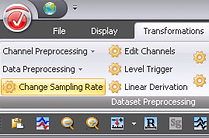
Go to Transformations >> Change Sampling Rate
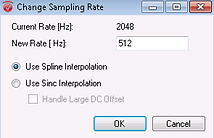
This opens the box below where you should select the required sampling rate (Hz). Choose "Use Spline Interpolation". Thereafter click on "OK". This will add a new (history) node underneath the participant's Raw Data.
TIP:
New history nodes will always inherit the specific BVA transformation applied to the data. In this case "Change Sampling Rate". It's recommended to rename all transformation nodes such that they include more specific info that characterized your analyses, as well as label condition differences. In this case, we could rename this node into "downsample_512Hz"
Filtering
For details on the settings of this step, please see the online manual for EEG preprocessing.
You can filter the data for analysis of IBIs with the settings below.
Go to Transformations >> Data Filtering >> IIR Filters
Select the settings as shown below:

Create ECG channel
This procedure allows you to generate a new channel based on the activity of other channels.
Go to Transformations >> Linear Derivation
This will open the Linear Derivation box that shows a table with columns (channels). The rows represent the values that indicate which channels have been involved in the subtraction. In the first column, you can enter the name of the new channel that you'd like to create. In the example below, we've created three new channels (HEOG, VEOG, and ECG). But if you are only interested in creating a new ECG channel, you can ignore the HEOG and VEOG channels in the image below.
You can directly specify the number of channels that you'd like to create by entering a value in the box "Number of Channels". If you click on "Refresh" the number of rows will change accordingly.
Make sure that you tick the box "Keep old channels" if you need the existing channels in the dataset, if analysing ECG data is of sole interest, you can untick the box Keep Old Channels.

Important:
Make sure to delete the old channels that were used to generate the new channel(s) via this procedure. You can do so using the following tool:
Go to Transformations >> Edit Channels
Untick all the old channels and other channels that you don't longer need and click OK.
Add R-markers
Now that you've isolated the ECG channel you can use the EKG marker solution to place R-markers on the R-tops in the ECG time-series. These R-markers will be used later on to calculate the Inter-Beat-Intervals (IBIs).
Go to Solutions >> EKG Markers

With the EKG marker solution, you can use BVA to place a variety of markers corresponding with the traditional peaks in a single heartbeat. For our IBI analyses we only focus on the R markers.
Select the ECG channel (if other channels exist)
Depending on whether your R peaks are associated with positive or negative values in the ECG, you choose Positive or Negative. The option Automatic also works in most cases, but using Positive or Negative polarities often works better.
You can untick all boxes under Marker Options, except for the R-markers.
Running the EKG marker solution often takes a while, The images below displays the before/after result.


Inspection of R-markers
To make sure the R-markers have been placed correctly, you should manually inspect the ECG time-series. If R-markers are misplaced or omitted from the data, you can adjust or place new markers manually via the Edit Marker option.
Click on the "M" icon in the toolbar.
This opens an interactive mode to adjust/add markers.

Segmentation (feedback-dependent IBI-markers)
The next step is to segment the ECG data surrounding stimuli of interest. Typically you'll focus on feedback-related IBI-changes. Thus segmenting on feedback stimuli would be the way to go.
Prior to isolating the feedback segments, you may want to include other stimuli or responses. In the example below, we first segment on 4 cues. And thereafter we segment on the feedback stimuli that follow the cues.
We can furthermore include specific requirements (Boolean expression) to make sure that some other stimuli or responses are either present or absent in the segments.
An important prerequisite for IBI segments is that they should be long enough to accommodate a large number of IBIs. For feedback-related IBI-analyses you need at least two IBIs prior to the onset of the feedback stimuli, and about 4 IBIs after the feedback stimuli.
In the example below we have first created 16 seconds segments with a short baseline.
Go to Segment Analysis Functions and choose Segmentation

Choose to create new segments based on a marker position

Choose the stimuli you want to use for segmentation (you can choose multiple stimuli if needed)

Choose the start and end time of the segment. Time 0 refers to the onset of the marker stimuli

In the example below, we have segmented a second time, but this time around the onset of the feedback stimuli. Note the inclusion of a Boolean expression, which in this case would exclude any feedback segments that include a response R144 within the interval -3100 to 0 (thus 3100 ms prior to the onset of the feedback stimulus

The last step is to define the length of the segment. Here we included 3500 ms prior to the onset of the feedback stimuli and 6500 ms after the feedback stimulus. Generally, this should include at least 2 IBIs before feedback onset and 4 IBIs after feedback onset. But it's recommended to carefully inspect your own data to define your ideal segment length. Longer segment length often comes at the expense of the number of trials.

Changing R-markers to feedback-related IBI-markers
Now that you've created feedback segments, the R-markers need to be renamed to markers that define their position relative to the feedback stimulus. You can use the following BVA-macro script (developed by dr. Henk van Steenberg). You can download the script here.
When opening this macro in BVA, the first lines of code refer to the number of R-peaks prior to and after the feedback stimuli. You can define these yourself, depending on your research interest. In the example below you can see we identified 3 markers prior and 5 markers after the onset of the feedback stimulus

Link IBI-markers to ECG data
We will use a peak-to-peak export function to calculate the distance in ms between two consecutive IBIs. to use this export function we first need to link the IBI marker to the ECG data. This can be done via the Edit marker (automatic mode) option.
Go to Transformations >> Choose "Edit Markers" under Data Preprocession

Choose the option "Automatic"

Next, you'll need to change the existing R-peak markers that were added to the data using the Macro.
>> Select the R-peak marker under "Choose Marker Type"
>> Select All descriptions under "Choose Marker Description"
>> Ender the word Peak under "New Marker Type"
>> Select the ECG channel under "Choose Channel"
>> Click on "Add" to add the command.
In the example below, we've also removed the existing R markers (created with the EKG solution), but this step is optional

Export IBI-markers
Now you can use BVA's peak-to-peak option to export the actual IBIs (i.e., the time interval between two consecutive heart beats) relative to a feedback stimulus.
Go to Solutions >> Export and choose Peak Export

Via the Peak Export solution can should define Peak2Peak as Peak action, and enter the peaks for comparison under Peak 1 and Peak 2. The settings as shown in the image below allow for using this option in a batch analyses (via a history template).

The peak-to-peak data will be exported to your BVA Export folder. This will include the peak-to-peak data for each participant and for all segments per condition. You will need to average these data per condition per participant for all the segments, You can use this R-script to do so.